SVM regression (SVR) vs Linear Regression

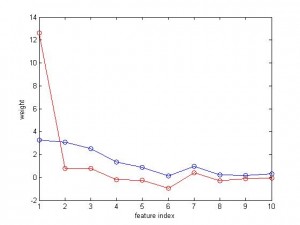
One particular nice thing about SVR is that the weight of each feature reflects the feature’s true contribution. If some features are highly correlated (this is common in neuroimaging data – e.g. adjacent voxel activity are very similar), you expect that the corresponding weights to be similar. SVR exactly does that. Linear regression, on the other hand, will give big weight to the feature which is best correlated to the dependent variable (y). Here is a demonstration in MatLab.

In the following simulation, we have 10 features which are highly correlated (see figure below).

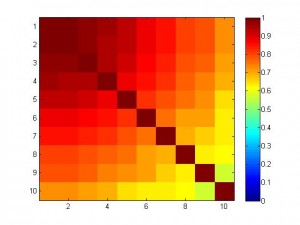
And the variable to be predicted is fairly nicely correlated with the features. Below I plotted the weight of 10 features. The blue curve is for SVR, and the red is for linear regression. As you can see, the weight for SVR is smooth and balanced, but the weight for regression is like ‘winner takes all’, the 1st feature has a big weight but others very small.

Here are the source code in MatLab. normalize.m can be found at https://www.alivelearn.net/?p=1083

N = 1000;
M = 1;
t = randn(N,1);

clear r
m = 10;%1:10:100;
for M = m
x = [t];
for ii=1:M-1
    x = [x  t+ii*randn(N,1)/10];
end

x = normalize(x);

% t1 = randn(N,1);
% t2 = randn(N,1);
% x = [t1 t2];
% y = 3*t1 - 5*t2;
y = 2*t + randn(N,1)/2 + 0;

% corrcoef([x y]);
%
% b= glmfit(x,y);
for ii = 1
    for jj=1
        tic;model = svmtrain(y(1:N/2),x(1:N/2,:),['-s 4 -t 0 -n ' num2str(ii/2) ' -c ' num2str(1)]);toc
        tic;zz=svmpredict(y(N/2+1:end),x(N/2+1:end,:),model);toc
        tmp = corrcoef(zz, y(N/2+1:end));
        r(M) = tmp(2);
    end
end

w = model.SVs' * model.sv_coef;
b = -model.rho;
b1 = [w]

% regression
b2 = glmfit(x(1:N/2,:), y(1:N/2,:));
yy = x(N/2+1:end,:)*b2(2:end) + b2(1);
b2 = b2(2:end)

sum((zz - y(N/2+1:end)).^2)
sum((yy - y(N/2+1:end)).^2)

end

figure('color','w');imagesc(corrcoef(x));colorbar
caxis([0 1])
figure('color','w');plot(b1,'o-');hold on;plot(b2,'o-r');xlabel('feature index');ylabel('weight')

return

hold on;plot(m, r, 'ro-');xlabel('# of dimension'); ylabel('r')
figure('color','w');plot(m, r, 'ro-');

figure('color','w');plot(x(1:N/2,:), y(1:N/2), 'b.');
hold on;plot(x(N/2+1:end,:), zz, 'r.');
xlabel('x')
ylabel('y')
legend({'training','test'})

%figure('color','w'); plot(zz, y(N/2+1:end), '.'); axis equal;axis square;
%figure('color','w'); plot(zz - y(N/2+1:end), '.')

---

---

---

写作助手，把中式英语变成专业英文

---

AI writing papers with real references

---

Want to receive new post notification? 有新文章通知我