The statistics toolbox in MatLab provides an easy way to do 1-way and 2-way anova. Below are some examples.
The functions are called anova1 and anovan. 1 way anova is to test if the mean in each group is same; and 2-way anova is to test (1) if the mean in each group is same, (2) if there is any interactions
1-way anova
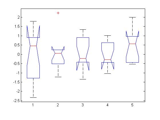
In the first example, there is no difference between means:

As expected, the p value is big (>0.05):
Source      SS      df     MS       F     Prob>F
------------------------------------------------
Columns    1.6778    4   0.41946   0.44   0.7804
Error     43.089    45   0.95753
Total     44.7668   49
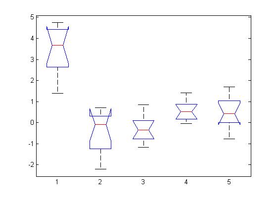
In the 2nd example, the 1st group has a larger mean

As expected, the p value is small
Source      SS      df     MS        F        Prob>F
-------------------------------------------------------
Columns    98.787    4   24.6969   36.94   1.10911e-013
Error      30.083   45    0.6685
Total     128.871   49
2-way anova
Let’s say we measured the height of 10 students. 5 of them are males, 5 of them has skin color ‘red’. We want to know if the height of male students is different from female students, if ‘red’ students is different from ‘blue’ students, and if the two factors have interactions (meaning the effect of gender on height is dependent on skin color).
Example 1: if the height only depends on gender, then we expect the pvalue for gender is small; p value for color or color*gender interaction is big.
  Source         Sum Sq.   d.f.   Mean Sq.     F     Prob>F
-----------------------------------------------------------
  gender         44.7625    1     44.7625    50.95   0.0004
  color           0.0389    1      0.0389     0.04   0.8403
  gender*color    0         1      0          0      0.9996
  Error           5.2709    6      0.8785
  Total          51.3893    9
Example 2: if the height depends on gender + color, then we expect the pvalue for gender and color is small; p value for color*gender interaction is big.
  Source         Sum Sq.   d.f.   Mean Sq.     F     Prob>F
-----------------------------------------------------------
  gender          67.444    1     67.4436    66.71   0.0002
  color           57.215    1     57.2151    56.59   0.0003
  gender*color     0.628    1      0.628      0.62   0.4606
  Error            6.066    6      1.011
  Total          162.43     9
Example 3: if the height depends on gender * color, then we expect the pvalue for gender and color is big; p value for color*gender interaction is small.
  Source         Sum Sq.   d.f.   Mean Sq.     F     Prob>F
-----------------------------------------------------------
  gender          0.0144    1      0.0144     0.02   0.8984
  color           0.0007    1      0.0007     0      0.9768
  gender*color   32.0284    1     32.0284    39.37   0.0008
  Error           4.8811    6      0.8135
  Total          36.9267    9
The source code:
% This is to test ANOVA in MatLab (stat toolbox)
% Xu Cui
% 2012/11/17

%% 1-way anova

% assume our data have 5 groups, and they draw from the same distribution

X = randn(10,5); % each column is a group
p = anova1(X) % As expected, p > 0.05

% assume our data have 5 groups, and the 1st group has a larger mean

X = randn(10,5);
X(:,1) = X(:,1) + 3;
p = anova1(X) % As expected, p < 0.05

% assume our data have 5 groups, and each group has a different mean

X = randn(10,5);
X = X + repmat([1:5], 10,1);
p = anova1(X) % As expected, p < 0.05

%% 2-way anova

% assume we have two factors, one is 'gender', taking values male(1) and
% female(0), the other skin color, taking value 'red' (1) and 'blue'(0). Then we
% measure the subjects' height.

gender = [ones(5,1); zeros(5,1)]; % first 5 are male
color = [1 0 1 0 1 0 1 0 1 0]';

% assume height only depends on gender
height = gender*5 + randn(10, 1) + 160;
p = anovan(height, {gender color}, 'model',2, 'varnames',{'gender';'color'})

% assume height depends on gender + color

height = gender*5 + color*5 + randn(10, 1) + 160;
p = anovan(height, {gender color}, 'model',2, 'varnames',{'gender';'color'})

% assume color and gender has interaction

height = [1 0 1 0 1 1 0 1 0 1]'*3 + randn(10, 1) + 160;
p = anovan(height, {gender color}, 'model',2, 'varnames',{'gender';'color'})


Dear Xu,
Great post, thanks. I was wandering what is with that red cross above the second group in the first figure. I searched the web with no avail 🙂 Do you happen to know what it means? It does not mean that the groups are significantly different and it appears even if one is only using first level anova.
Cheers
Interesting observation. I don’t know it either.
Xu
Hello Xu Cui and Anon, the red cross indicates an outlier, a datapoint which is further than 2 or 3 standard deviation from the group mean (depending on the way the graph is plotted, see matlab reference for details).
I can confirm Vaaal’s outlier interpretation; it seems to be a feature of Matlab’s boxplot function. It’s very useful if you are performing sanity checks on variables.
Hi all,
According to Statistics Toolbox, the plus sign at the top of the plot is an indication of an outlier in the data. This point may be the result of a data entry error, a poor measurement or a change in the system that generated the data.
By default, each outlier is a value that is more than 1.5 times the interquartile range away from the top or bottom of the box.
hi all
how can i calculate coefficient of regression model and thier significance using matlab for quadratic model
thanks