[last updated: 2009/06/15]
Also check out NIRS data analysis (GLM and visualization)
Environment requirement
- MatLab
- SPM
- xTopo under xjView
xjview is located in/fs/fmrihome/fMRItools/Xjview
Add xjview to path byaddpath(genpath('/fs/fmrihome/fMRItools/Xjview'))
xTopo is based on topo program provided by Hitachi. It is modified by me. You can download xTopo at https://www.alivelearn.net/nirs/xtopo.zip
Preparation
- convert NIRS data file to csv format using ETG4000 program.
- copy the 3D positioning data (00X.pos).
- If you don’t have 3D positioning data, you may use the template channel positions located in
xjview/nirs_data_sample/?x??.pos
Procedure
- In MatLab command window, run
topo
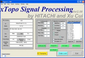
- Click button “Data Load” and select the data csv file. You only need to select the 1st (or left) file if you use 4×4 or 3×5 bilateral configurations. After a pause you will find the data information (such as subject name and marker timing etc)
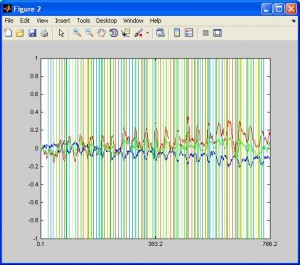
- To view the overall time series, click button “Continuous Hb”. You will see the HbO, HbR and total traces for each channel. Colorful vertical lines indicates marker timing. To see more detailedly the trace of a certain channel, enter the channel number in CH box and click button “Zoom”.
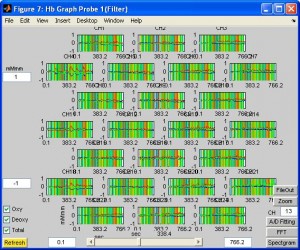
- To see activation in a topographic view, click on any channel. You can also see the animation by click button “Play”.
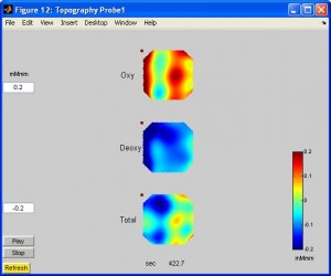
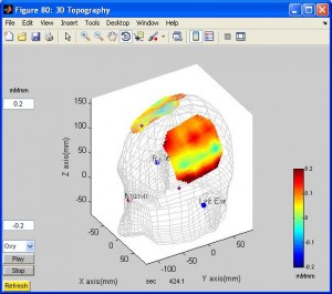
- To see activation in 3D topo, in xTopo main window click “3D Topography”. You need to select the ???.pos file. You can rotate the brain.
- To average time series across trials, you need to select the markers (event) you are interested in (by clicking button “Select Mark”) and input proper parameters for Pre time, relax time and post time, then click either button “Integral Hb” or “cuixu Integral Hb” (I will explain the difference later).
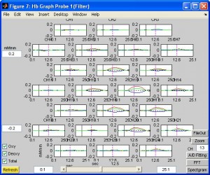
- You can also zoom, plot topo, 3D topo like what you do for continuous time series.
Explanations
- The difference between “Integral Hb” (IH) and “cuixu Integral Hb” (cH):
IH: cut and collect the time series for each occurence of the event. Then do detrending based on pre time and post time for each individual time series. Finally average across occurences. Both pre and post time parameters are important.
cH: Do detrending/smoothing with filter pass for the entire time series first, then cut and collect the time series for each occurence, then average. Pre time, relax time and post time is used when cutting the time series. The data used is from (Pre time) seconds before event onset, to (Relax + Post time) seconds after onset. Relax and Post time are not that important. As long as the sum is the same, the result won’t change. - Obtaining the data used in plot: You will find a variable called hb_data in the workspace. It contains the data used to plot. It’s an array. The 1st one is for probe set 1, 2nd for set 2. raw means raw data and fil means filtered data. The first dimension is hb species (oxy, dxy and total), second is time, 3rd is channel.
>> hb_data(1)
ana_mode: 2
calc_flg: 2
raw: [3x251x24 double]
fil: [3x251x24 double]


I’m struggling to get your code running an Matlab 2010a. SPM is installed and in the path, as is xjview.m. yet I see this error:
??? Undefined function or method ‘passfilter’ for input arguments of type ‘double’.
Error in ==> cuixu_calc_int at 175
dsignal = passfilter(continuous_data(p_cnt).raw(1,:,hb_ch), [0.3 0.01],
10);
??? Error while evaluating uicontrol Callback
where does passfilter come from? Do I need any other packages installed? Any hints?
passfilter function is not included in the public version of xjview. Here is the function:
function y = passfilter(x, threshold, samplingFrequency)
% function y = passfilter(x, threshold, samplingFrequency)
% low or/and high pass filter
%
% x: orginal signal
% threshold: the frequency thresholds. It should be an array of length 2.
% The first component corresponds to the low pass filter threshold and the
% 2nd one corresponds to the high pass threshold. If you don’t want to
% set the threshold, put nan.
% samplingFrequency: the sampling frequency of the original signal x.
% Default 10 Hz
%
% y: the result signal
%
% Note: this script needs signal toolbox
%
% Example:
% y=humps([0:.01:1])+randn(1,101)*10;
% figure;plot(y)
% hold on; plot(passfilter(y, [0.5, nan], 10), ‘r’)
%
% Xu Cui
% 2007-10-02
if nargin < 2 error('At least two arguments are required.'); end if nargin < 3 samplingFrequency = 10; end if ~isfinite(threshold(1)) && ~isfinite(threshold(2)) y = x; return end if isfinite(threshold(1)) && isfinite(threshold(2)) [b,a]=ellip(4,0.1,40,[threshold(2) threshold(1)]*2/samplingFrequency); elseif isfinite(threshold(1)) [b,a]=ellip(4,0.1,40,[threshold(1)]*2/samplingFrequency); elseif isfinite(threshold(2)) [b,a]=ellip(4,0.1,40,[threshold(2)]*2/samplingFrequency, 'high'); end y = filtfilt(b,a,x); return
thanks for the passfilter function. it seems though there are some more functions missing (now choking on ellip and Maximize).
Also there is a little glitch when running on a Unix system (case-sensitive filesystem) – in input_para.m you try to fopen a file ‘ALL_E_coef.txt’ but after unziping xtopo.zip it is called All_E_coef.txt (lower case Ls).
Do you plan on releasing an xjview version that has the needed functions?
Thanks again for your help!
ellip function is in MatLab’s signal processing toolbox and not part of xjview. Maximize function is from http://www.mathworks.com/matlabcentral/fileexchange/10274-maximize-figure-windows
We will eventually release the tools when they are stable.
I am trying to load my data sampled from fNIRS machine which has .csv
However each time I try it, I get this error :
Error in load_ad_etg7000 (line 25)
load_flg = 0;
Output argument “ad_data” (and maybe others) not assigned during call to
“C:\Users\AhmetCakir\Desktop\MRes\SPM8\cuixuTSP\load_ad_etg7000.m>load_ad_etg7000”.
Error in load_ad (line 81)
[info, ad_data, mark,para,para_p] =
load_ad_etg7000(fname,MainFigure,para,para_p,para_h,dis_no);
Error in OnDataLoad (line 64)
[info,ad_data,mark,para,para_p] =
load_ad(strcat(pname,fname),MainFigure,para,para_p,para_h,dis_no);
Error while evaluating uicontrol Callback
I cannot understand why I have this error.
I have cross checked it with the sample data that you have provided and could not see any differences. Could you please let me know why I am getting this kind of error ?
Thanks
I created the csv file from the Hitachi’s own program. I remembered that once I tried to change the csv file and then it failed. So I guess you have to create the csv in Hitachi’s way.
I have problems with fileOut, it doesn’t save measurements data into the file. Only the information about subjects.
any ideas?
thanks
Hi Dr. Xu Cui,
I wonder if you have a paper reference for your “cuixu Integral Hb”?
Thanks,
Guoqing
@Guoqing
We do not have a paper referencing this button/function.
I want to make an animated visualization with the output file of ETG4000, so Is it still available to use xTopo to fulfill the animated visualization ?
I want to download the file in the website: https://www.alivelearn.net/nirs/xtopo.zip
But it’s an invalid website.
The link is updated and is valid now.
Thanks for replying ^^
Excuse me,
May I ask how do you create the .pos file in your sampling data?
Which instrument(Ex: ISOTRAK II) and software(Ex: Brainstorm) did you use to create the .pos file?
Thanks for replying