updated: 2010/01/05, add plot of original data
Assume our data contains two features and they are highly correlated (say, r>0.9). The 1st feature does slightly better than the 2nd one in classifying the data. The question is, is the weight of the 2nd feature close to 0, or close to the weight of 1st feature?
If this is a linear regression, we know the winner (1st feature) will take all — the beta value for the 2nd feature will be close to 0. But in linear SVM, the weight for the 2nd feature seems close to the weight of 1st feature.
Here is the result of simulation. In this simulation, feature 1 classify the data well (97% accuracy). The 2nd feature is simply the 1st feature plus different amount of noise. We can see that when feature 1 and feature 2 are highly correlated, their weights are close in SVM. But in linear regression the weight of the 2nd feature remains close to 0 b/c it doesn’t add any classification power in addition to feature 1.
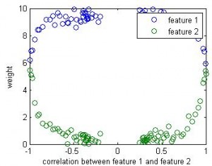
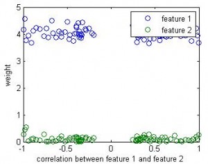
Updated: original data plot with different correlation
The data are generated this way:
N = 500;

l = [ones(N,1); -ones(N,1)]; % label

d = [];

d(:,1) = l + randn(2*N,1)/2;

d(:,2) = sign(rho)*d(:,1) + randn(2*N,1)/10*rho;

d = normalize(d);
rho is a parameter controlling the amount of noise added to the 2nd component. Its range is between -100 to 100. Note data is normalized (so all data point are between 0 and 1) prior to further analysis (SVM or linear regression).
For SVM, I use libsvm 2.89 MatLab version. I used linear SVM with C=1.
For linear regression, I simply use the most naive method:
beta = inv(X'*X)*X'*Y;
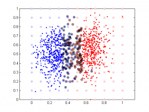
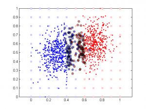
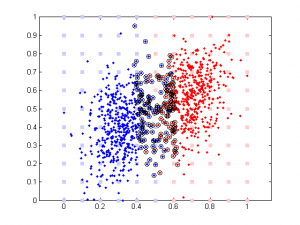
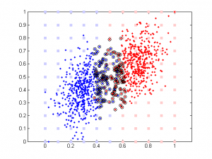
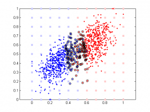
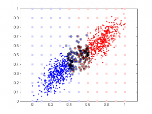
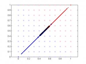



It’s very interesting to see the tendency in SVM results plot, esp. when the correlation is low. Since that means the distribution of your data is more spherical than elliptical, but the high ratio between the two weights means the support vectors are located at sides of two distributed ‘clouds’, even their centers might be located diagonally. In the case of linear regression, supposing you used a direct glm solution (or regularized solving procedure?), I would expect a big variance when the two feature components are highly correlated, as the covariance matrix is almost singular (a strong regularization should lead to results similar to the svm case though).
It would be really nice to see more detail about your experiment setting, including data generation and parameters used in two analyses.
Thank you, etude. More details are added.